Neil C. Bruce
	Main Page Surface Scattering Capacitance Volume Scattering Polarization Cursos

Vector electromagnetic scattering from rough surfaces with infinite gradients

Vector wave scattering from 2D rough surfaces can be calculated using theStratton-Chu equation

where Esur and Hsur are the electric and magnetic surface fields, respectively, and . The term ksc is the scattered wave vector, r´ is a point on the surface and dS´ is a segment of the surface area.

It can be shown that the terms inside the integral can be written

where e is the direction of the incident electric field, t is the vector which is perpendicular to the local plane of incidence at each point of the surface and kinc is the incident wave vector. The subscripts V and H are the vertical and horizontal polarizations respectively.

The Kirchhoff approximation applied to the case of vector electromagnetic scattering through the Stratton-Chu equation involves replacing the exact surface fields Esur and Hsur with the sum of the incident and reflected electric and magnetic fields at each point of the surface. The normal vector is written in terms of the increments in x, y and the height increments in these two directions.

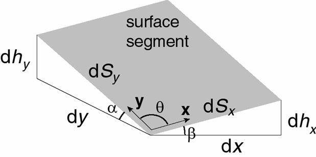
The geometry of a single surface segment for the 2D rough surface case is shown above. The vectors x and y, the vectors along the side of the surface segment, can be written in terms of their coordinates as

and the normal to the surface segment is given by

or

The normalizing factor of this vector can be written as

where dS is the area of the surface segment and is the variable term over which the integral in the Stratton-Chu equation is performed. This gives finally

It can be seen that substitution of this equation in the Stratton-Chu equation will give three integrals (as compared with two integrals for the case of a 1D surface). If, for example, a surface segment has dx = 0, i.e. a vertical wall parallel to the y-axis, only the first integral of variables will contribute to the total scattered field giving the correct contribution for this part of the surface.

Examples of the results obtained with this method is shown below.

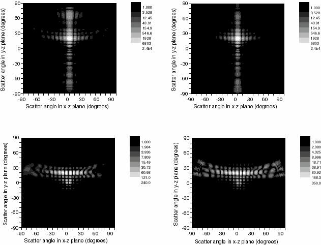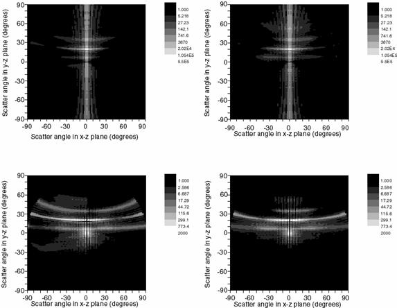
	3D log scale intensity maps of the light scattered from a single groove in a plane. Top left: HH scattering; top right: VV; bottom left: HV; bottom right: VH. Surface parameters: L = 10l, a = 4l and d = 0.5l. The incidence angle is qinc = 20°.
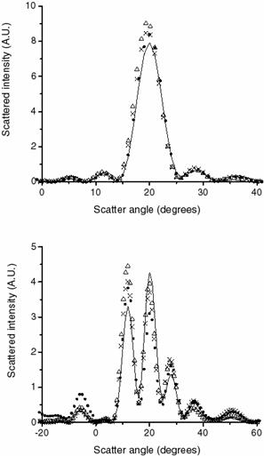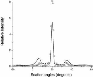
	Cross-sections through the graphs for d = 0.5l (top) (this is the case shown in the graphs above) and d = 1.75l (bottom) for polarization HH (indicated by the crosses) and the VV polarization curves for the same cases (open triangles) compared with the 2D Kirchhoff results for the same cases(points) and the integral equation results (full curves).
	3D log scale intensity maps of the light scattered from 4 grooves in a perfectly conducting plane. Top left: HH scattering; top right: VV; bottom left: HV; bottom right: VH. Surface parameters: average groove width 2l, with a rectangular probability distribution of width 1l; average groove depth 2l, with a rectangular probability distribution of width 1l; and average groove separation (end of one groove to the start of the next) 2l, with a rectangular probability distribution of width 1l. The incidence angle is qinc = 20°
	Cross-sections through the graphs shown above for polarization HH in (indicated by the crosses) and the VV polarization curves for the same case (open triangles) compared with the 2D Kirchhoff results for the same cases (full curves).

Publications

• N.C. Bruce, "Scattering from high-sloped surfaces using the Kirchhoff approximation", Proceedings of SPIE, vol. 4780, (2002), 1-6.
• N.C. Bruce, "Scattering from infinitely sloped surfaces by use of the Kirchhoff approximation", Applied Optics, 42, (2003), 2398-2406.
• N.C. Bruce, "Calculations of the light scattered from an infinite-sloped surface using the Kirchhoff approximation", Proceedings of SPIE, vol. 5622, (2004), 1550-1555.
• N.C. Bruce, "Control of the backscattered intensity in random rectangular-groove surfaces with variations in the groove depth", Applied Optics, 44(5), (2005).